Parallelizing neural networks on one GPU with JAX

Most neural network libraries these days give amazing computational performance for training large neural networks. But small networks, which aren’t big enough to usefully “fill” a GPU, leave a lot of available compute unused. Running a small network on a GPU is a bit like buying an apartment building and then living in the janitor’s closet.

In this article, I describe how to get your money’s worth by training dozens of networks at once. As you follow along, we’ll efficiently train dozens of small neural networks in parallel on a single GPU using the vmap function from JAX. Whether you are training ensembles, sweeping over hyperparameters, or averaging across random seeds, this technique can give you a 10x-100x improvement in computation time. If you haven’t tried JAX yet, this may give you a reason to.

All of this was originally implemented as part of my library for evaluating representations, reprieve. If you’re interested in learning about the pitfalls of representation learning research and how to avoid them, I wrote a blog post on that too.

If you’re just here for the code, there’s a colab that has what you need.

• The difficulty of accelerating small networks
• Large batches fill GPUs but learn worse
• Training more networks in parallel
  • Automatic batching with JAX and vmap
  • A first draft of parallel network training with vmap
• Bootstrapped ensembles
  • A bootstrapped data sampler
  • Training the bootstrapped ensemble
• Conclusion

The difficulty of accelerating small networks

With the end of Moore’s Law-style clock speed scaling, modern high-performance computing platforms get good performance not by taking less time for a single operation, but by doing more in parallel. They are wider, not faster. This applies to accelerators like GPUs and TPUs, or even Apple’s new laptop SoCs.

The operations used in neural network training are pretty ideal for taking advantage of very wide architectures. Large matrix multiplies consist of huge numbers of smaller operations that can be executed at the same time. On top of that, we always use minibatch training, where we compute a loss gradient on tens, hundreds, or thousands of examples in parallel, then average those gradients to estimate the “true” gradient on the dataset.

Modern automatic differentiation libraries like PyTorch are optimized for squeezing as much performance as possible out of a wide accelerator for these kinds of workloads. Train a ResNet-50 on your GPU and you’ll likely see GPU utilization numbers up near 100%, indicating that PyTorch is squeezing all the speed possible out of your hardware.

However, for training small networks, we run into fundamental limits of parallelization. To be sure, a two-layer MLP will run much faster than the ResNet-50. But the ResNet has about 4B multiply-accumulate operations, while the MLP has only 100K.¹ Much as we might like it to, our MLP will not train 40,000 times faster than a ResNet, and if we inspect our GPU utilization we can see why. Unlike the ResNet, which uses ~100% of the GPU, the MLP may only use 2-3%.

A simple explanation is that their computation graphs aren’t as wide as the GPU is. Glossing over a ton of complexity about data loading, fixed costs per loop, and how GPUs actually work, a small network with a reasonable batch size just doesn’t have enough parallelizable operations to use the entire GPU efficiently.

Large batches fill GPUs but learn worse

One way to use more compute in parallel would be to increase the batch size. Instead of using batches of, say, 128 elements, we could crank that up until we fill the GPU. In fact, why not use the entire dataset as one batch and parallelize across every element!

On MNIST, we can actually try this. With a batch size of 128, we see GPU utilization at ~2% and a speed of about 11s / epoch. By caching the entire dataset in GPU memory and performing full-batch gradient descent (i.e. using the whole dataset as one batch), we can get up to a frankly disturbing 0.01s / epoch with 97% GPU utilization!

Unfortunately, this doesn’t correspond to faster learning; the resulting model only has 79% test accuracy, compared to 98% for our small-batch model. I was lazy and didn’t bother to adjust any hyperparameters, and assuredly we could squeeze out a bit more performance with careful tuning. However, as a rule we don’t expect very large batch gradient descent to yield performance that’s as good as small batch.²

Even ignoring issues of generalization error, large batches aren’t very computationally efficient for most problems. A theoretical argument against very large batches comes from a classic paper by Bottou & Bousquet.³ We can think of a full-batch gradient descent update as being very accurate, but computationally expensive, and a small-batch update as being highly approximate, but very cheap. Bottou & Bousquet show that taking lots of approximate updates results in much faster learning than taking fewer accurate updates.

While using very large batches can definitely saturate our GPU, they don’t actually help us train a small network any faster. So what can we do instead?

Training more networks in parallel

We can’t train a small network much faster on our current hardware, at least not without any exotic tricks. If we’re careful to make sure our data loading is quick, we can probably train our two-layer MLP 400x faster than a ResNet-50. And that’s pretty fast! But we’re still leaving an additional 100x improvement on the table, at least according to our ballpark estimate that the ResNet uses 40,000x as much compute.

What should we do with the whole rest of our GPU? Well, in practice we often don’t just want to train one neural network. We might want to run with many random seeds to be confident in our results, or we could sweep over different hyperparameter settings, or we could even train a bootstrapped ensemble of networks for higher accuracy. Instead of waiting for our first network to finish training before starting the next, we could run all of these experiments at the same time!

The simplest version of this is to run our training script multiple times, putting several copies of (almost) the same job on the same GPU. This works, and has the advantage of flexibility: those jobs don’t have to have anything in common, they just have to stay within the memory budget of the GPU. It treats your GPU like a tiny cluster, agnostic to the content of the job scripts. However, this deployment strategy has a lot of overhead: you get multiple Python processes, multiple copies of the library on the GPU, multiple data transfer calls between CPU and GPU… the list goes on. In practice you can run a few small jobs on one GPU, but you’ll run out of GPU memory and clog your GPU before you get to 100.

Instead we’re going to see how to avoid duplicating work for our computer by writing an ordinary training step function, then using JAX to batch the computation over many neural networks at once.

Automatic batching with JAX and vmap

A lot has been written about JAX in the past, so I’ll give only a cursory introduction. JAX is an exciting new library for fast differentiable computation with support for accelerators like GPUs and TPUs. It is not a neural network library; in a nutshell, it’s a library that you could build a neural network library on top of. At the core of JAX are a few functions which take in functions as arguments and return new functions, which are transformed versions of the old ones. It also includes an accelerator-backed version of numpy, packaged as jax.numpy, which I will refer to as jnp. For more I’ll refer you to Eric Jang’s nice introduction, which covers meta-learning in JAX, and the JAX quickstart guide.

On to a quick summary of the core functions in JAX that we’ll use, along with the arguments we care about:

jax.jit(fun, ...): Takes a function fun and returns a faster version. There’s more to it than this, but enough for our purposes.

jax.grad(fun, ...): Takes a function fun and returns a function that computes its gradient with respect to (by default) the first argument. For example, we could define g = jax.grad(lambda x: x**2), and then use it by calling g(2). In essence, what we did was:

1. Define $f(x) = x^2$ using a lambda expression.
2. Make a new function $g = \frac{df}{dx}(x) = 2x$.
3. Evaluated $g(2) \rightarrow 4$.

jax.vmap(fun, in_axes=0, ...): Takes a function fun and returns a batched version of that function by vectorizing each input along the axis specified by in_axes. vmap is short for vectorized map; if you’re familiar with map in other programming languages, vmap is a similar idea.

Under the hood vmap does basically the same thing that you would if you were vectorizing something by hand. For instance, suppose we had a PyTorch function def f(a, b): torch.mm(a, b) that applies to matrices, but we are given a batch of matrices at a time. We could compute the answer with a for loop, but it would be slow. Instead we can look up the batched PyTorch function which computes batched matrix multiply (it’s bmm), and define the function def vf(a, b): torch.bmm(a, b). We have transformed f by hand into a vectorized version, vf.

In JAX we can do the same thing automatically using vmap. If we had a function def f(a, b): jnp.matmul(a, b), we could simply do v = jax.vmap(f). Crucially, this doesn’t just work for primitive functions. You can call vmap on functions that are almost arbitrarily complicated, including functions that include jax.grad.

One subtlety here is in the use of in_axes. Say that instead of taking a batch of a and a batch of b, we wanted a version of our function f that takes a batch of a, but only a single b, and gives us back jnp.matmul(a[i], b) for each a[i]. We can define this new function v0, which is vectorized only with respect to argument 0, with the following call: v0 = jnp.vmap(f, in_axes=(0, None)). This asks that argument 0 of f be vectorized with respect to axis 0, and argument 1 not be vectorized at all. Our result will be the same as if we iterated over the first dimension of a, and used the same value of b each time.

A first draft of parallel network training with vmap

Now that we have the basics of JAX, we can start implementing a parallel training scheme. The basic idea is simple: we will write a function that creates a neural network, and a function that updates that network, and then we’ll call vmap on them. For full code please refer to the colab that accompanies this post.

I’ve defined a simple classification dataset: two spirals in 2D. We can control the amount of noise in the data and how tight the spiral is.

def make_spirals(n_samples, noise_std=0., rotations=1.):
    ts = jnp.linspace(0, 1, n_samples)
    rs = ts ** 0.5
    thetas = rs * rotations * 2 * np.pi
    signs = np.random.randint(0, 2, (n_samples,)) * 2 - 1
    labels = (signs > 0).astype(int)

    xs = rs * signs * jnp.cos(thetas) + np.random.randn(n_samples) * noise_std
    ys = rs * signs * jnp.sin(thetas) + np.random.randn(n_samples) * noise_std
    points = jnp.stack([xs, ys], axis=1)
    return points, labels

points, labels = make_spirals(100, noise_std=0.05)

For our neural network, we can create a simple MLP classifier in Flax, a neural network library built on top of JAX:

class MLPClassifier(nn.Module):
    hidden_layers: int = 1
    hidden_dim: int = 32
    n_classes: int = 2

    @nn.compact
    def __call__(self, x):
        for layer in range(self.hidden_layers):
            x = nn.Dense(self.hidden_dim)(x)
            x = nn.relu(x)
        x = nn.Dense(self.n_classes)(x)
        x = nn.log_softmax(x)
        return x

Because JAX is a functional language, we will carry around the state of a network separately from the functions that update or use that state. Neural network libraries in JAX are still something of a work in progress and the abstractions aren’t terribly intuitive yet. Somewhat confusingly, instantiating a Flax nn.Module returns an object with some automatically-generated functions, not a neural network state. A full description of how this works is available in the Flax docs, but for now you can gloss over anything to do with Flax.

We can instantiate our model functions, then define a couple of helper functions for evaluating our loss. Here value_and_grad is a JAX function that acts like jax.grad, except that the function it returns will produce both $f(x)$ and $\nabla_x f(x)$.

classifier_fns = MLPClassifier()

def cross_entropy(logprobs, labels):
    one_hot_labels = jax.nn.one_hot(labels, logprobs.shape[1])
    return -jnp.mean(jnp.sum(one_hot_labels * logprobs, axis=-1))

def loss_fn(params, batch):
    logits = classifier_fns.apply({'params': params}, batch[0])
    loss = jnp.mean(cross_entropy(logits, batch[1]))
    return loss

loss_and_grad_fn = jax.value_and_grad(loss_fn)

We’re ready now to create functions to make, train, and evaluate neural networks.

def init_fn(input_shape, seed):
    rng = jr.PRNGKey(seed)                                     # jr = jax.random
    dummy_input = jnp.ones((1, *input_shape))
    params = classifier_fns.init(rng, dummy_input)['params']   # do shape inference
    optimizer_def = optim.Adam(learning_rate=1e-3)
    optimizer = optimizer_def.create(params)
    return optimizer

@jax.jit  # jit makes it go brrr
def train_step_fn(optimizer, batch):
    loss = loss_fn(optimizer.target, batch)
    loss, grad = loss_and_grad_fn(optimizer.target, batch)
    optimizer = optimizer.apply_gradient(grad)
    return optimizer, loss

@jax.jit  # jit makes it go brrr
def predict_fn(optimizer, x):
    x = jnp.array(x)
    return classifier_fns.apply({'params': optimizer.target}, x)

This provides the entire API we’ll use for interacting with a neural network. To see how to use it, let’s train a network to solve the spirals! Here we’re using the entire dataset of (points, labels) as one batch. Later we’ll deal with proper data handling.

model_state = init_fn(input_shape=(2,), seed=0)
for i in range(100):
    model_state, loss = train_step_fn(model_state, (points, labels))
    print(loss)

-> 0.011945118

Unsurprisingly, this works pretty well.

If our hypothesis is correct, we can plug these functions into vmap and be embarrassingly parallel! We will use in_axes with vmap to control which axes we parallelize over. In our init_fn, which takes the input shape as an argument, we want to use the same input shape for every network, so we set the corresponding element of in_axes to None. For now all of our networks will update on the same batch at each step, so in defining parallel_train_step_fn we parallelize over the model state, but not over the batch of data: in_axes=(0, None). The number of random seeds we feed in to parallel_init_fn will determine how many networks we train, in this case 10.

parallel_init_fn = jax.vmap(init_fn, in_axes=(None, 0))
parallel_train_step_fn = jax.vmap(train_step_fn, in_axes=(0, None))

K = 10
seeds = jnp.linspace(0, K - 1, K)

model_states = parallel_init_fn((2,), seeds)
for i in range(100):
    model_states, losses = parallel_train_step_fn(model_states, (points, labels))
print(losses)

-> [0.01194512 0.01250279 0.01615315 0.01403342 0.01800855 0.01515956
 0.00658712 0.00957206 0.00750575 0.00901282]

Great! We can train 10 networks all at once with the same code that used to train one! Furthermore, this code takes almost exactly the same amount of time to run as when we were only training one network; I get roughly a second for each run, with the parallel version being faster than the single run as often as not.⁴ We can also bump K up higher to see what happens. On my Titan X, training 100 networks still takes the same amount of time as training only one! This basically delivers our missing 100x speedup:

We can’t train one MLP 40,000x as fast as a ResNet, but we can train 100 MLPs 400x as fast as a ResNet.

If you’re just here for speed, you’re done! By passing a different seed to initialize each network with, this procedure will train many different networks at once in a way that’s useful for evaluating things like robustness to parameter initialization. If you’d like to do a hyperparameter sweep, you can use different hyperparameters for each network in the network intitialization. But if you’re interested in getting more out of this technique, in the next section I describe how to use parallel training to learn a bootstrapped ensemble for improved uncertainty calibration.

Bootstrapped ensembles

If we plot the predictions for two of the networks we just trained, we see something interesting:

Try to spot the differences in these predictions. Super hard, right? Even though we’ve trained two different neural networks, because they were trained on the same data, their predictions are almost identical. In other words, they’re all overfit to the same sample of data.

In this section we’ll see an application of parallel training to learning bootstrapped ensembles on a dataset. Bootstrapping is a way of measuring the uncertainty that comes from only having a small random sample from an underlying data distribution. Instead of training multiple networks on exactly the same data, we’ll resample a “new” dataset for each network by sampling with replacement from the empirical distribution (AKA the training set).

Here’s how this works. Say we have 100 points in our dataset. For the first network, we create a new dataset by drawing 100 samples uniformly at random from our existing dataset. We then train the network only on this newly-sampled dataset. Then for the next network, we again draw 100 samples from the real training set, and we train our network #2 on dataset #2, and so forth for however many we want. In this way, each network is trained on a dataset that’s slightly different; it may have many copies of some points, and no copies of others.

Bootstrapping has the nice property that the randomness in the resample decreases as the dataset grows larger, capturing the way a model’s uncertainty should decrease as the training set more fully describes the data distribution. For small datasets, having 0 versus 1 sample of a particular point in the training set will make a huge difference in the learned model. For large datasets, there’s probably another point right next to that one anyway, so it doesn’t matter too much if you leave out (or double) any one point.

A bootstrapped data sampler

The crucial change from our previous setup is that, on every training step, each network is going to get a different batch of data. To implement this, we will write a bootstrapped sampler which we can vmap. Each time we call the vmapped sampler, we’ll get back a batch of batches of shape (number_of_networks, batch_size, data_size). The layout will basically be

[minibatch from dataset 0,
 minibatch from dataset 1,
 ...,
 minibatch from dataset K-1]

where dataset 0 is the first bootstrapped resample we took from our original dataset. Ideally we want to implement this function without duplicating the entire dataset $K$ times in memory.

To do this, we will stop thinking directly about indices in the dataset, and start thinking about random seeds. Imagine we want to sample one point uniformly at random from a dataset. We could use a call like

point_index = jr.randint(jr.PRNGKey(point_seed), shape=(),  # jr = jax.random
                         minval=0, maxval=dataset_size)

to choose an index in our dataset to return. This is a pure function of the point_seed that we use. In mathematical terms, it is a surjection of the larger space of all possible random seeds onto the smaller space of integers in the interval [0, dataset_size]. Visually it looks something like this:

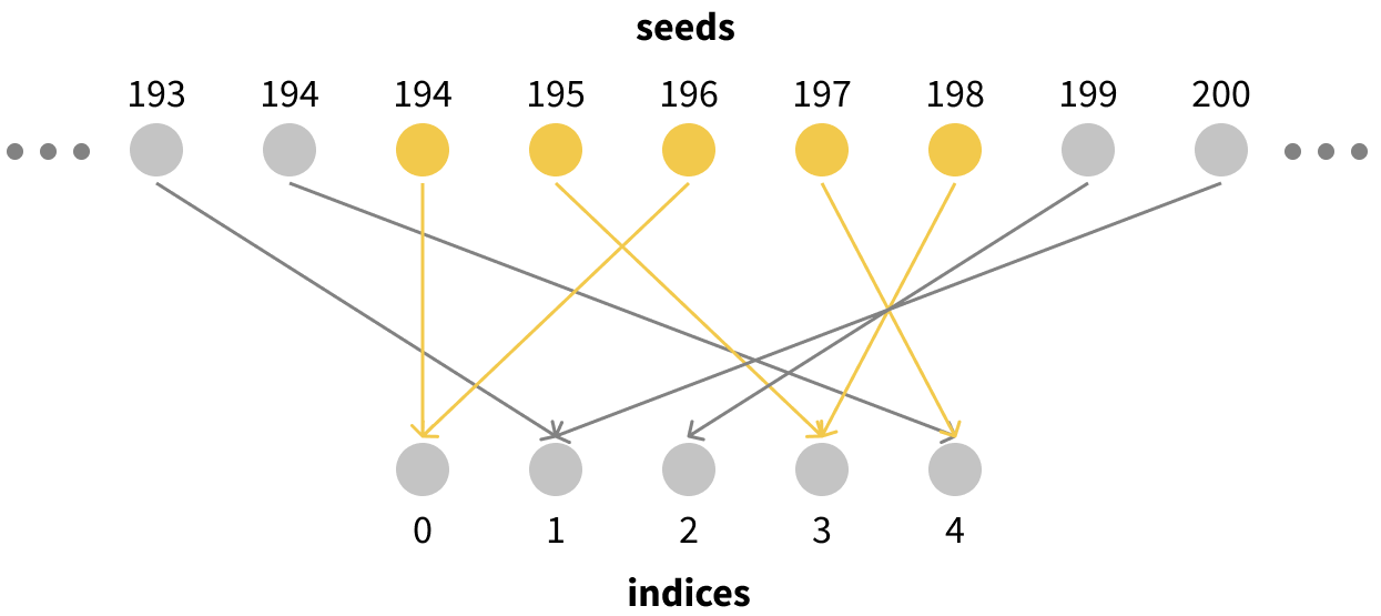
This has a super useful property for us: since every individual seed corresponds to an index sampled uniformly at random, any set of $N$ seeds corresponds to a bootstrapped sample of indices of size $N$! For example, if we were to take seeds 194-198, they would correspond to exactly the kind of bootstrapped resampling of our size-5 dataset that we want. We would have 2 copies of data points 0 and 3, no copies of points 1 or 2, and one copy of point 4.

All we need to do to generate a bootstrapped resample of a dataset of size $N$ is to pick some seed $i$ to start from and use all the seeds in $[i, i + N - 1]$ to sample indices. What we need is a function which maps from a dataset_index, which tells us which bootstrapped dataset we’re sampling from, to the first random seed which will be included in our resample. Since I’m lazy, I’ll use the hash function in jax.random.split.⁵

def get_first_seed(dataset_index):
    return jr.split(jr.PRNGKey(dataset_index))[0, 0]

get_first_seed(0)

-> DeviceArray(4146024105, dtype=uint32)

Great! We got some giant random number. This should be reassuring; the only way this could go wrong is if somehow we picked values of $i$ which were too close to each other. This would make it so that e.g. dataset #1 had seeds $[i, i + n - 1]$, and dataset #2 had seeds $[i + 3, i + n - 2]$; since the seeds overlapped, the samples of those datasets would be too correlated. The fact that we’re drawing from a really large space makes this astronomically unlikely.

Now we can use this function to implement a new function which will fetch us point $i$ from resample $k$:

@jax.jit
def get_example(data_x, data_y, dataset_index, i):
    """Gets example `i` from the resample with index `dataset_index`."""
    first_seed = get_first_seed(dataset_index)
    dataset_size = data_x.shape[0]

    # only use dataset_size distinct seeds
    # this makes sure that our bootstrap-sampled dataset includes exactly
    # `dataset_size` points.
    i = i % dataset_size

    point_seed = first_seed + i
    point_index = jr.randint(jr.PRNGKey(point_seed), shape=(),
                             minval=0, maxval=dataset_size)
    # equivalent to x_i = data_x[point_index]
    x_i = jax.lax.dynamic_index_in_dim(data_x, point_index,
                                       keepdims=False)
    y_i = jax.lax.dynamic_index_in_dim(data_y, point_index,
                                       keepdims=False)
    return x_i, y_i

And with this we can write a function which, given a dataset and a list of the bootstraps we want to sample from, gives us an iterator over batches-of-batches:

def bootstrap_multi_iterator(dataset, dataset_indices):
    """Creates an iterator which, at each step, returns a batch of batches.

    The kth batch is sampled from the bootstrapped resample of `dataset`
    with seed `seeds[k]`."""

    batch_size = 32
    dataset_indices = jnp.array(dataset_indices)
    data_x, data_y = dataset
    dataset_size = len(data_x)

    get_example_from_dataset = jax.partial(get_example, data_x, data_y)

    # for sampling a batch of data from one dataset
    get_batch = jax.vmap(get_example_from_dataset, in_axes=(None, 0))
    # for sampling a batch of data from _each_ dataset
    get_multibatch = jax.vmap(get_batch, in_axes=(0, None))

    def iterate_multibatch():
        """Construct an iterator which runs forever, at each step returning
        a batch of batches."""
        i = 0
        while True:
            indices = jnp.arange(i, i + batch_size, dtype=jnp.int32)
            yield get_multibatch(dataset_indices, indices)
            i += batch_size

    loader_iter = iterate_multibatch()
    return loader_iter

Training the bootstrapped ensemble

Thanks to the flexibility of the JAX API, switching from training $K$ networks on one batch of data to training $K$ networks on $K$ batches of data is super simple. We can change one argument to our vmap of train_step_fn, construct our iterator, and we’re ready to go!

# same as before
parallel_init_fn = jax.vmap(init_fn, in_axes=(None, 0))
# vmap over both inputs now: model state AND batch of data
bootstrap_train_step_fn = jax.vmap(train_step_fn, in_axes=(0, 0))

# make seeds 0 to N-1, which we use for initializing the network and bootstrapping
N = 100
seeds = jnp.linspace(0, N - 1, N).astype(jnp.int32)

model_states = parallel_init_fn((2,), seeds)
data_iterator = bootstrap_multi_iterator((points, labels), dataset_indices=seeds)
for i in range(100):
    x_batch, y_batch = next(data_iterator)
    model_states, losses = bootstrap_train_step_fn(model_states, (x_batch, y_batch))
print(losses)

-> [0.14846763 0.09306543 0.24074371 0.26202717 0.26234168 0.18515839
 0.10521372 0.11991201 0.1059431  0.10932036]

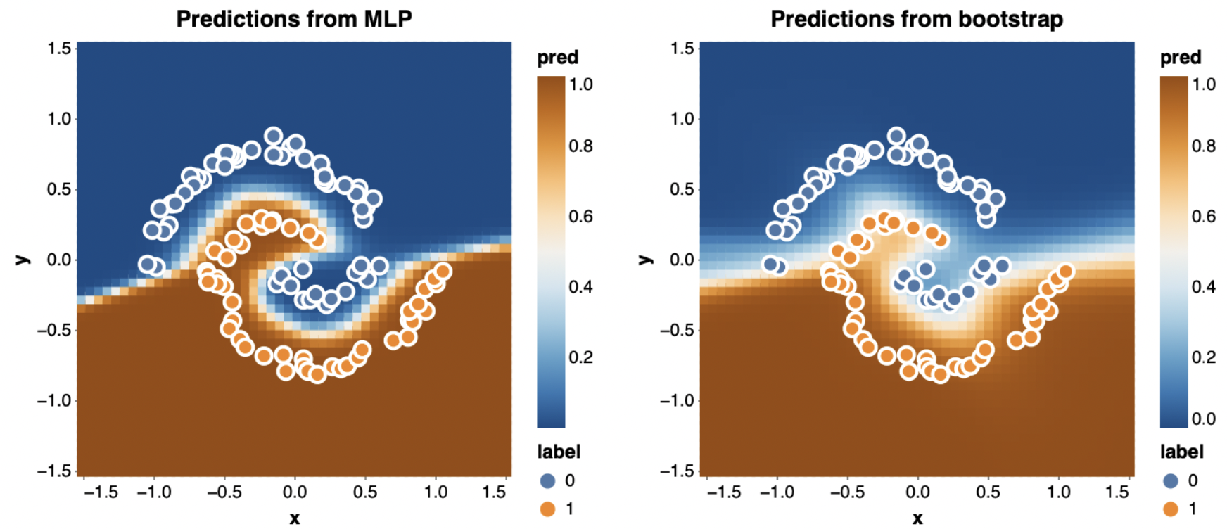
Naturally, this still takes only about a second. Visualizing the predictions of a couple of the bootstrapped networks shows that they’re way more different than when we trained each one on the whole dataset.

I’ve plotted the entire dataset on top of the predictions, even though each network may not have seen all those points. In particular, in the plot on the right it seems likely that the points which are currently misclassified were not in that network’s training set.

The exciting thing we can use these bootstrapped networks for is uncertainty quantification. Since each network saw a different sample of the data, together their predictions can tell us what parts of the space are sure to be classified one way and which are more dependent on noise in your training set sample. To do this, I simply average the probabilities I get from each network:

The results are really striking when we compare against the single network we trained on all the data before (shown at left):

The single network predicts labels for almost the entire space with absolute confidence, even though it was only trained on 100 points. By contrast, the bootstrapped ensemble (right) does a much better job of being uncertain near the boundary between the classes.

Conclusion

Practically anytime you’re training a neural network, you would rather train several networks. Whether you’re running multiple random seeds to make sure your results are reproducible, sweeping over learning rates to get the best results, or (as shown here) ensembling to improve calibration, there’s always something useful you could do with more runs. By parallelizing training with JAX, you can run large numbers of small-scale experiments lightning fast.

Citing

If this blog post was useful to your research, you can cite it using

@misc{Whitney2021Parallelizing,
    author = {William F. Whitney},
    title = { {Parallelizing neural networks on one GPU with JAX} },
    year = {2021},
    url = {http://willwhitney.com/parallel-training-jax.html},
}

Acknowledgements

Thanks to Tegan Maharaj and David Brandfonbrener for reading drafts of this article and providing helpful feedback. The JAX community was instrumental in helping me figure all of this stuff out, especially Matt Johnson, Avital Oliver, and Anselm Levskaya. Thanks are also due to my co-authors on our representation evaluation paper, including Min Jae Song, David Brandfonbrener (again), Jaan Altosaar, and my advisor Kyunghyun Cho.